Building and Calibrating Noise Sources for 8970B
When a commercial noise source unexpectedly failed during a receiver project, I set out to determine whether a simple homemade noise source could be used with an HP 8970B Noise Figure Analyzer.
Along the way, I developed practical methods for estimating the Excess Noise Ratio (ENR) of an unknown source without a calibrated standard, calibrating DIY noise sources against a known standard, and evaluating measurement uncertainty caused by source mismatch.
For anyone building high-performance VHF and UHF receivers, preamplifiers, or front ends, noise figure is one of the most important performance parameters. Achieving the lowest possible noise figure often requires careful tuning and repeated measurements, which in turn demands a reliable and accurately calibrated noise source.
A Noise Source Failure Leads to an Experiment
While working on a 2-meter receiver front end, I suddenly found myself without a usable noise source. My ND3101 noise head, which had served faithfully for decades, simply stopped working. Given its 1990 date code and years of service, I couldn't really complain.
A replacement was immediately ordered, but I wasn't willing to put the project on hold while waiting for it to arrive. Fortunately, the work didn't require laboratory-grade accuracy. What I really needed was a way to compare noise performance while tuning the circuit.
That raised an interesting question. Could a simple homemade noise source provide useful measurements, and could its ENR be estimated well enough to make the HP 8970B useful until a replacement arrived?
Before diving into the solution, it helps to review a few fundamentals.
Noise Figure, Noise Factor, and ENR Demystified
Noise Factor (F) and Noise Figure (NF) describe how much a device degrades the signal-to-noise ratio passing through it. Noise Factor is defined as the ratio of input SNR to output SNR, assuming a standard source temperature of 290 Kelvin.
Since every real-world device adds some amount of noise, the output signal-to-noise ratio is always worse than the input ratio. As a result, Noise Factor is always greater than or equal to one.
Noise Figure is simply Noise Factor expressed in decibels:
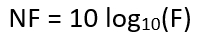
An ideal amplifier that adds no noise whatsoever would have a Noise Figure of 0 dB.
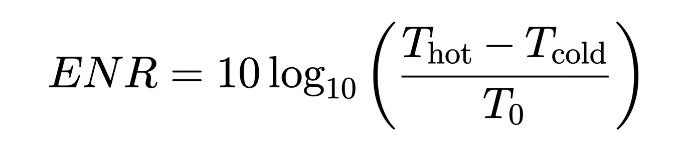
Modern noise figure analyzers use the Y-factor method to determine NF. This technique relies on a calibrated noise source whose output is characterized by its Excess Noise Ratio, or ENR. ENR describes the difference in noise power between the source's "hot" state and its "cold" state, referenced to the standard temperature of 290K.
By measuring the change in output power when the noise source switches between these two states, the analyzer can calculate the noise contribution of the device under test.
For cascaded systems, the importance of accurate measurements becomes obvious when considering Friis's formula. The first stage in the signal chain dominates overall system noise performance because the gain of that stage suppresses the contribution of noise generated by subsequent stages. This is why so much effort goes into optimizing the first low-noise amplifier in a receiver system.
Ultimately, the accuracy of any noise figure measurement depends on the accuracy of the ENR values assigned to the noise source. Any uncertainty in the ENR calibration contributes directly to uncertainty in the calculated noise figure.
Building a DIY Noise Source Test Fixture
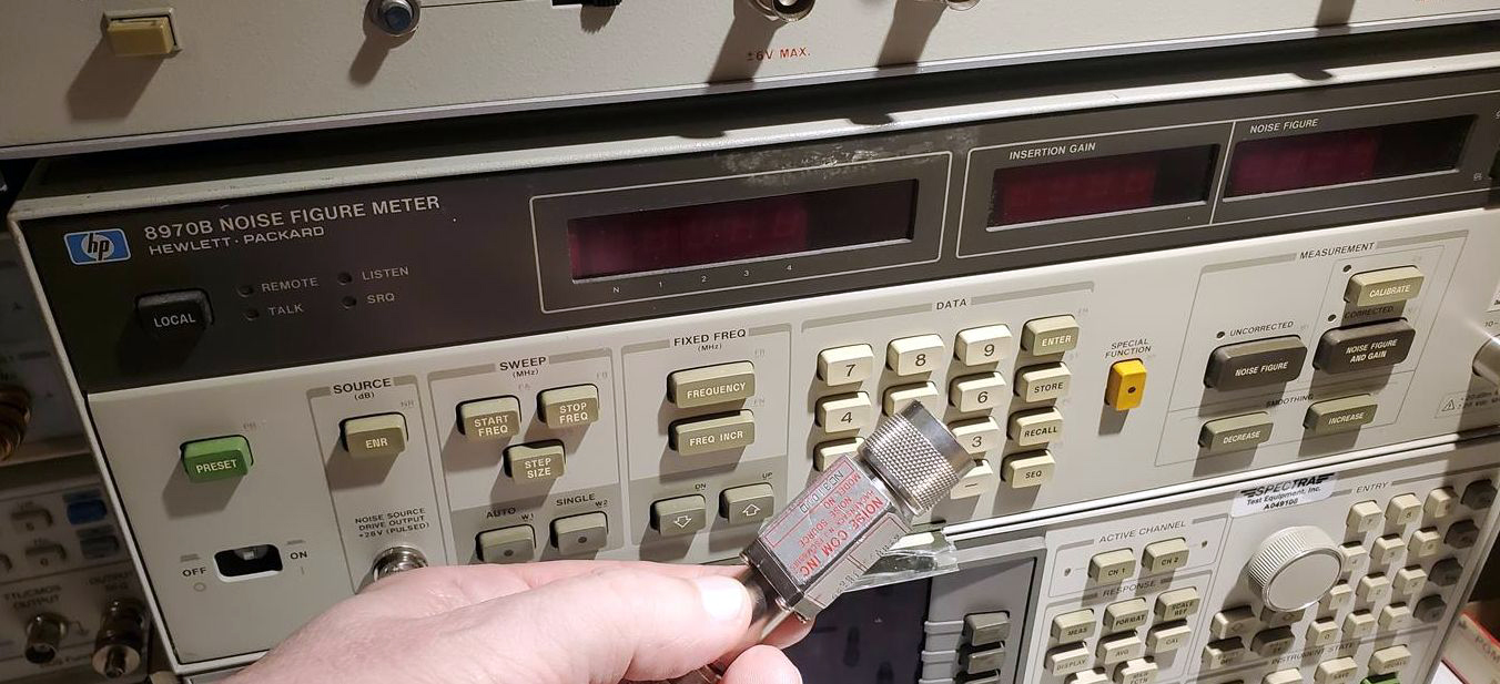
With no working commercial source temporarily available, I quickly assembled a simple broadband noise generator.
The design used a serial connected, reverse-biased PN junction operating in avalanche breakdown. Both reverse-biased transistor emitter-base junctions and certain Schottky diodes can produce useful broadband noise when operated beyond their normal reverse-bias region.
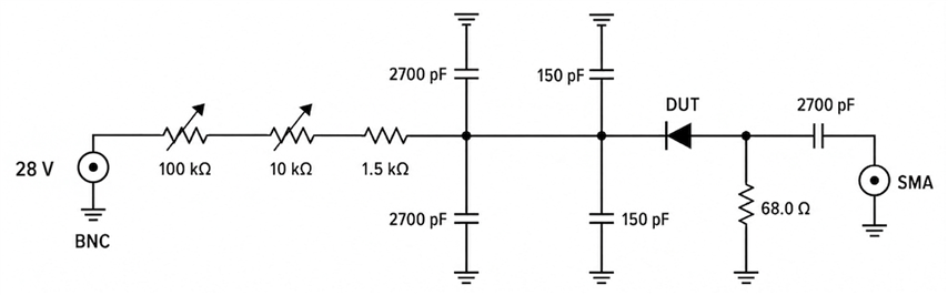
The noise source was to be powered directly from the HP 8970B's 28-volt pulsed drive output.
Several microwave and UHF devices from the junk box were evaluated. I intentionally avoided zeners and common transistors such as the 2N3904, as their relatively high junction capacitance limits useful bandwidth. Since I wanted coverage through the analyzer's full 1600 MHz range, low-capacitance RF devices were the logical choice.
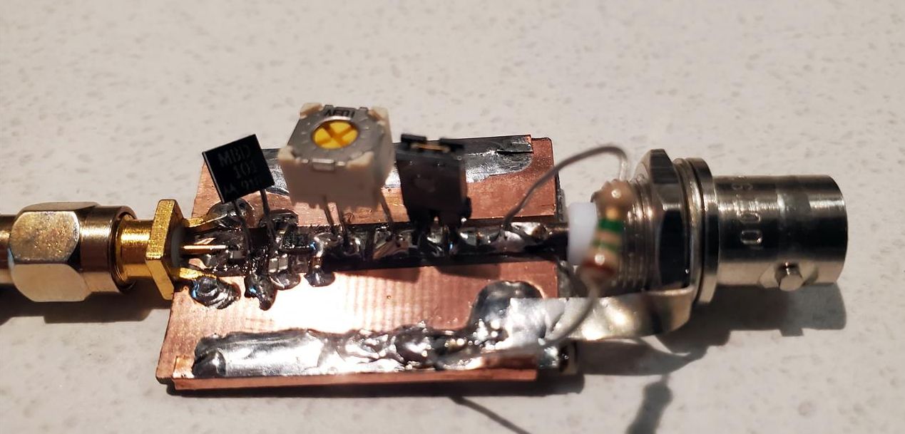
The test fixture was deliberately simple and allowed both rapid device changes and easy adjustment of operating current.
Evaluating Candidate Devices
Since the analyzer itself was not calibrated for the homemade source, I focused on measuring Y-factor rather than absolute ENR. In general, for a given analyzer a higher Y-factor indicates a higher ENR. Likewise, a flatter frequency response suggests a flatter ENR curve.
One of the first devices tested was the BFR93A, which has appeared in several amateur noise source designs. It produced plenty of noise but exhibited approximately 6 dB of roll-off by 1600 MHz. The BFG540/x proved more interesting. While it generated slightly less overall noise, its frequency response was considerably flatter and more consistent across the measurement range. Assuming a reasonably flat analyzer response, a flatter measured Y-factor suggests a flatter ENR characteristic.
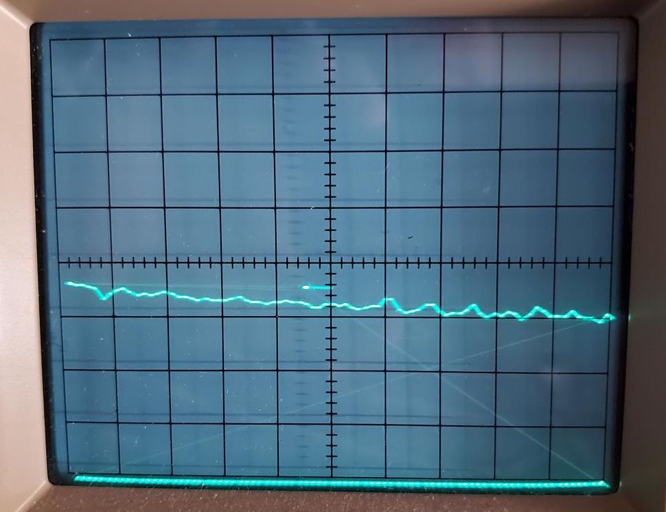
Measurements were made at various operating currents to determine how current affected noise output. Care must be taken here. Reverse-biased junctions gradually age when operated at excessive current densities. Over time, the avalanche process can alter the junction structure and change the device's noise characteristics. This effect is particularly important with modern microwave devices, whose junctions are extremely small.
Note the jitter present on the trace. Its pattern is highly repeatable across a wide range of devices and noise-source types, indicating that the effect originates primarily within the test fixture rather than the devices under test. This fixture was assembled as a rapid prototype using readily available components rather than parts specifically selected for broadband RF measurement applications.
Although surface-mount components were used throughout, the self-resonant frequencies (SRFs) of several capacitors and inductors likely fall within the measurement range. As these resonances are encountered, the resulting impedance variations produce localized perturbations in the measured Y-factor. Additional artifacts arise from broadband component parasitics, including package inductance, stray capacitance, and non-ideal ground-return paths, all of which become increasingly significant at higher frequencies. Minor standing-wave effects within the fixture and interconnecting transmission paths further contribute to the observed response irregularities.
The combined result is a series of small, repeatable anomalies that appear as trace jitter throughout the sweep. A purpose-built fixture employing components selected for higher SRFs, minimized parasitics, improved transmission-line geometry, and better impedance control would be expected to produce a noticeably smoother response.
For long-term stability, I recommend keeping operating current below about 3 mA. In practice, the lowest current that provides adequate noise output is usually the best choice.
Avalanche Noise Sources — Why They Behave So Inconsistently
Avalanche-based noise sources are deceptively simple in concept but notoriously variable in practice. While the underlying mechanism is impact ionization in a reverse-biased junction, the actual noise output depends strongly on device geometry, doping profiles, and local electric field distribution.
Two nominally identical devices can produce significantly different noise levels or spectral flatness. Even more subtly, the same device can shift behavior over time if operated at elevated current density, as microscopic changes in the junction alter the avalanche region.
This is why commercial noise diodes are carefully selected, characterized, and then “linearized” with precision attenuation. The diode itself is never the final source of the calibrated ENR — it is only the raw noise generator.
The Importance of Output Attenuation
The measurements described above were made with no attenuator connected to the source output. At that stage, I was merely comparing the raw noise output of candidate devices.
However, a practical noise source requires output attenuation. The reason is straightforward. A reverse-biased junction presents a different impedance when switched on and off. This means the source VSWR changes between hot and cold states, introducing significant uncertainty into noise figure measurements.
A broadband attenuator provides isolation between the noisy junction and the device under test, dramatically reducing mismatch effects. Many laboratory noise sources employ approximately 15 to 20 dB of output attenuation. The exact value represents a compromise between output match and usable ENR. For my purposes, 15 dB appeared to provide a reasonable compromise between isolation and available noise output, although, more is always better, as long the final ENR is adequate for purpose.
VSWR and Measurement Uncertainty
Impedance mismatch is often the largest source of error in noise figure measurements.
Whenever the noise source and DUT are not perfectly matched, reflections occur between them. Since the noise source exhibits different reflection coefficients in its hot and cold states, the actual noise power delivered to the DUT changes slightly as the source switches.
The analyzer interprets these changes as variations in ENR, leading to measurement error.
The theoretical uncertainty can be calculated from the source reflection coefficient and the DUT input reflection coefficient:
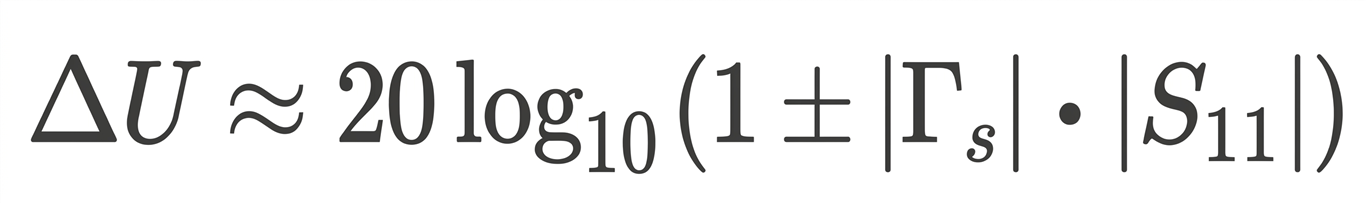
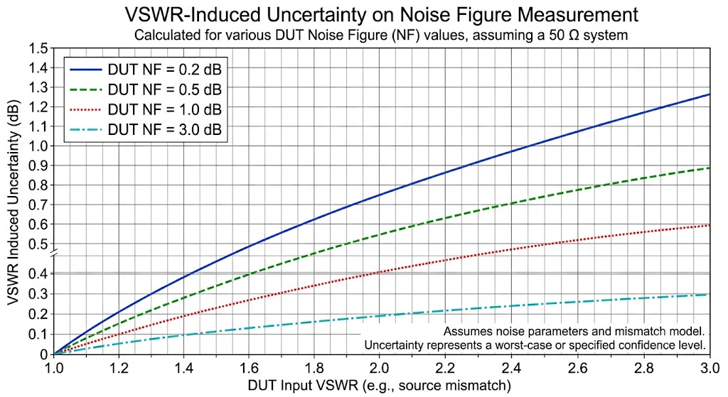
In routine measurements, the phase relationships are usually unknown, so VSWR values are used to establish worst-case limits. Even modest mismatches can have surprisingly large effects. A source and DUT with VSWRs of only 1.5:1 can easily introduce several tenths of a decibel of uncertainty.
For extremely low-noise amplifiers, the problem becomes severe. A 0.2 dB noise figure LNA measured through a mismatch of only 1.1:1 can exhibit uncertainty approaching 0.1 dB—half the value being measured. This is why serious sub-1 dB noise figure work demands high-quality attenuators and careful attention to source matching. The chart below depicts the effects of VSWR on a measurement:
Calibrating a Noise Source Without a Standard
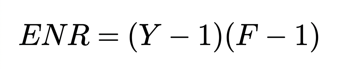
The next challenge was determining the ENR of the homemade source. Fortunately, there is a direct relationship between ENR, receiver noise factor, and measured Y-factor:
At this stage, all quantities are linear values rather than decibel values.
The HP 8970B measures Y-factor very accurately, even when the attached noise source is not calibrated. Performing a dummy calibration with the homemade source can make operation more convenient, but it does not affect the measured Y-factor.
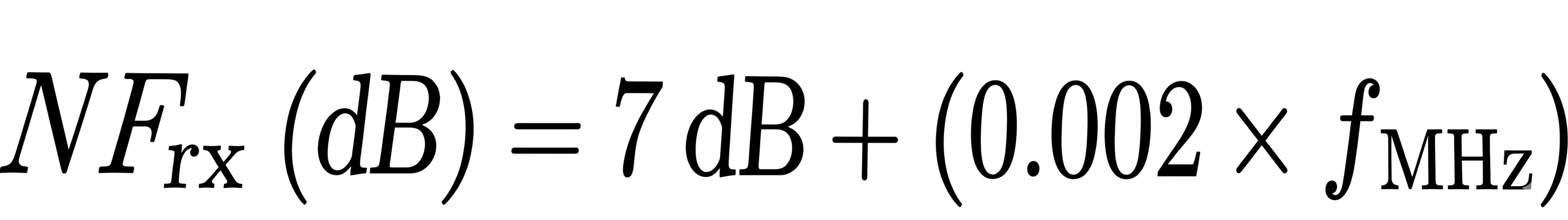
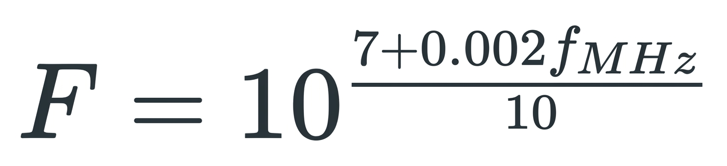
The remaining unknown is the noise figure of the analyzer itself. Fortunately, Hewlett-Packard characterized this parameter very well. HP characterized the internal receiver noise figure at approximately
where f is frequency in MHz. While not intended as a calibration standard, this approximation is sufficiently accurate for estimating the ENR of an unknown source.
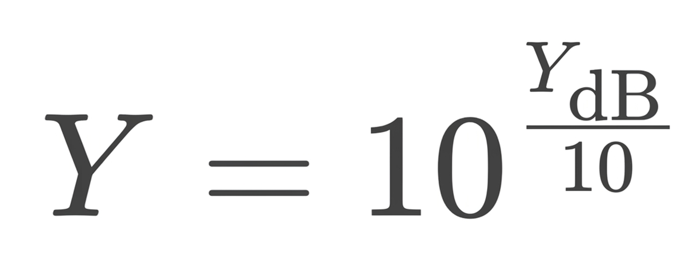
This approximation introduces the primary uncertainty in the calculation, but practical results are generally within about ±0.4 dB. If Y-factor is measured in decibels, convert it to linear form using:
Likewise, convert the analyzer noise figure to linear noise factor:
Alternatively, one can also work entirely in dB:

Once those values are known, ENR can be calculated. In my case, the BFG540 based source produced a measured Y-factor of approximately 19 dB, corresponding to an estimated ENR of about 25 dB. A few days later, when the replacement commercial source arrived, I was pleasantly surprised to discover that the estimate was remarkably close within 0.25 dB.
Not bad for a homemade source and a forty-year-old analyzer. The result also serves as a testament to the quality of HP's original noise figure receiver design and characterization.
Checking Used Noise Sources
This technique is useful for more than emergency measurements. Anyone purchasing a used noise source at a hamfest or from an online auction should consider performing a quick sanity check before trusting the calibration data.
Noise sources can be damaged by abuse, excessive current, or age-related degradation, and there is no simple DVM measurement that reveals such problems. Using the above method, a Y-factor check can quickly determine whether a source is reasonably close to its stated ENR.
Why the HP 8970B Became an Industry Standard
Introduced in the mid-1980s as an evolution of earlier HP noise figure meters, the 8970 series quickly became the reference platform for RF noise measurements in both industry and defense applications.
Its success came from combining automation, repeatability, and practical calibration handling in a way earlier analog systems could not match. The ability to store and interpolate ENR tables directly inside the instrument removed one of the largest sources of operator error in Y-factor measurements.
For decades, it served as the standard bench instrument for amplifier characterization from VHF through microwave frequencies, and even today remains widely used in amateur, academic, and repair environments due to its robustness and measurement transparency.
Although modern analyzers offer faster interfaces and wider frequency coverage, few match the simplicity and predictability of its measurement model.
Calibrating DIY Sources Against a Known Standard
After experiencing one noise source failure, I decided it would be wise to keep a couple of calibrated backups on hand.
My replacement commercial source provides approximately 15 dB ENR. Since the homemade sources produce considerably more noise, I planned to add attenuators to create additional 10 dB and 5 dB ENR sources while providing good return loss. In addition, I maintain a separate calibration table for my primary commercial source when used with a dedicated 10 dB attenuator that reduces its ENR to approximately 5 dB. This will take all four of 8970B’s available ENR tables.
The higher raw ENR of the homemade source should not be interpreted as superior performance; commercial noise heads intentionally sacrifice ENR through precision attenuation in order to achieve excellent source match and calibration stability.
For very low-noise devices, a lower ENR source often provides a better overall tradeoff between mismatch uncertainty and measurement repeatability. While reducing ENR decreases mismatch sensitivity, it also reduces the Y-factor and therefore increases statistical measurement uncertainty. In practice, ENR values around 5 dB are often preferred when measuring sub-1 dB noise figure amplifiers.
The calibration procedure is surprisingly simple:
First, enter the ENR table of the calibrated source into the HP 8970B and perform a normal calibration. Allow at least 30 to 60 minutes of warm-up time and use generous averaging for best results. I recomment using at least 32x averaging on your 8970.
Once calibration is complete, the analyzer should indicate approximately 0 dB noise figure across the frequency range.
Now substitute the new, DIY source. The displayed noise figure directly indicates the ENR difference between the calibrated source and the new one. The relationship is:
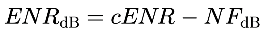
where cENR is the calibrated ENR (in 8970 ENR table) and NFdb is the displayed noise figure.
If the new source produces more noise than the calibrated source, the displayed noise figure will be negative. When an additional attenuator is added to tailor the ENR, the relationship becomes:
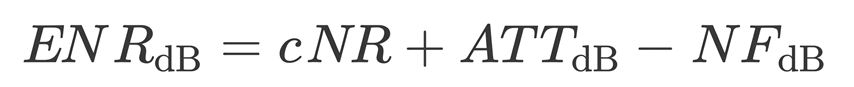
This makes it easy to determine the attenuation required to create a source with any desired ENR value.
Temperature Effects
All calculations assume the noise source OFF state is near the standard reference temperature of 290 K. Significant departures from room temperature introduce additional uncertainty into the estimated ENR.
The HP 8970B Architecture — Why It Still Works So Well
The HP 8970B is fundamentally a ratio-measurement system built around a highly stable IF receiver and precision logarithmic detection. Its strength is not exotic RF design, but disciplined metrology architecture.
At its core, the instrument performs synchronized power measurements of the DUT output while switching a calibrated noise source between hot and cold states. The internal processing then removes second-stage contributions and applies stored ENR data to solve directly for noise figure.
A key advantage of the design is that ENR correction is frequency-aware and table-driven, allowing accurate measurements across a wide RF range without recalibration of the instrument itself.
Despite its age, the architecture remains effective because it separates RF uncertainty (noise source + DUT) from measurement linearity (receiver + detector), which is exactly the correct way to structure a metrology instrument.
Conclusion
The HP 8970B remains one of the most useful pieces of test equipment ever built for low-noise RF work. Even decades after its introduction, it continues to provide excellent results when paired with a properly characterized noise source.
Perhaps more importantly, the analyzer's accurate Y-factor measurements make it possible to estimate, verify, and calibrate noise sources without access to a metrology laboratory. A simple homemade avalanche noise source can be surprisingly effective for development work, troubleshooting, and even as a backup standard.
While nothing replaces a professionally calibrated noise source for precision measurements, the techniques described here allow experimenters to continue working when a commercial source is unavailable, verify the health of used equipment, and create practical secondary standards for the home laboratory.
In the spirit of amateur radio, sometimes understanding the measurement is just as valuable as making it.
This article is reprinted with permission of the author, Christopher Krstanovic - AI2F.
About Author
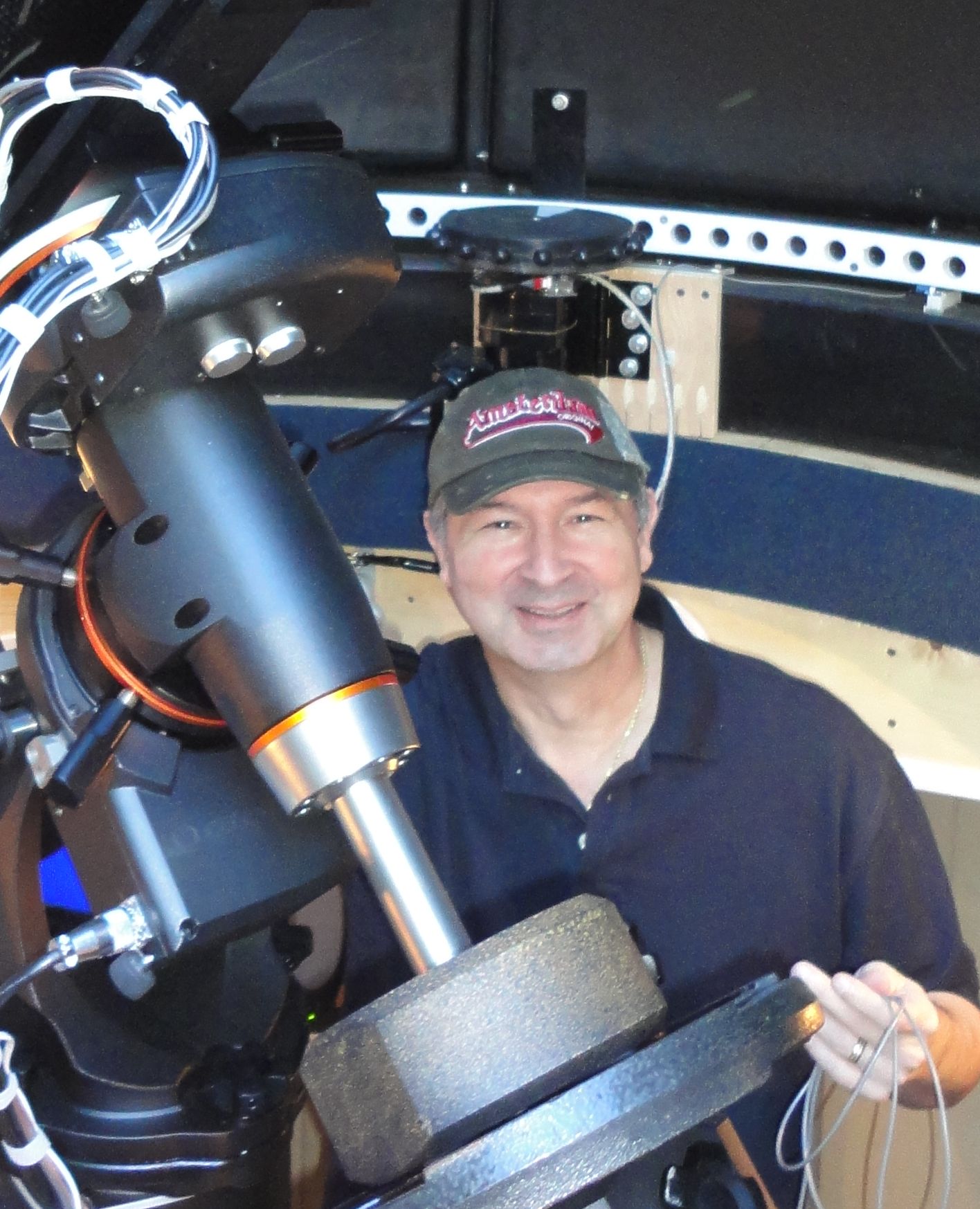 Christopher Krstanovic, AI2F, is a lifelong amateur radio operator, first licensed in the US in 1980s as WR1F. He holds degrees in Physics and a PhD in Electrical Engineering, and his career has spanned corporate engineering as well as technology entrepreneurship. After leaving corporate America, he founded and led three companies before returning to active amateur radio under his current call sign. His operating interests include HF, antenna design, practical radio engineering and Astronomy.